Seeing the World Through Images: A Sneak Peek into Image Processing Techniques

“Images save the past & retain the memories,
Make us relive the forgotten stories,
All emotions trapped in frames,
From happiness to sorrow & joy to pain.”

The life style of people has changed remarkably in last few decades, and its credit has to go to hard work of scientists and engineers. The revolution in field of electronics has not only miniaturized electronic devices, but also has improved their performance incredibly. The most common example is: Revolution in mobile phones.

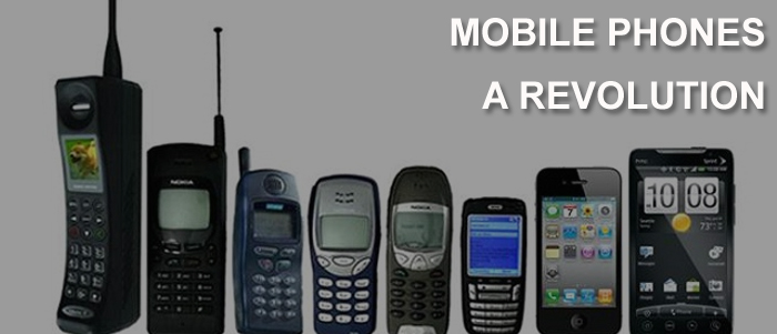This has happened in just last 15 years. From heavy, big & dull phones which were only capable of making calls, we have reached to era of smart phones, which are like portable computers and have features like music player, camera, games & different kinds of apps that can perform thousands of tasks.

These days with the easy access to smart phones, culture of taking pictures and posting it on social websites is at its peak. We all use our phone cameras and its various features, like, auto focus, High Dynamic Range (HDR) imaging, blurring, image transformations, night mode, image mosaic etc, without  thinking much about its working.

This article gives insight about various image processing techniques and the way they affect the image. We would be discussing about images and various image transforms, followed by simple applications of image processing like image registration, image mosaicing and few methods of 3D reconstruction from images.

Image processing has brought great advancement to humankind. It has saved lives in the form of MRI and other medical imaging techniques. It has improved the agricultural and maritime practices by remote sensing. And of course, the value of using digitally enhanced images to recreate memories and entertainment industry to increase joy of life cannot be overstated.

Image processing is an essential part of computer vision & plays a critical role in advancement of artificial intelligence. Various image processing techniques work together with deep learning in order to tackle the major problems faced by Artificial Intelligence, like, object recognition, pattern recognition, microscopic imaging, future prediction etc. This will improve surveillance and tackling terror threats by leaps and bounds. This will also help in fundamental research in countless other fields and having further impact on people’s lives.

What is an image?

For normal person, image is a reproduction or imitation of the form of a person or thing. In order to represent this imitation, we discretize the image in smaller blocks, called pixel and assign them some numbers related to intensity and colour at the corresponding point in object.  Pixels are the smallest addressable element in an all point addressable display device. Hence, for someone involved in image processing, image is nothing but just a matrix of numbers. If it’s gray scale image, it would be a 2D matrix and if it’s a coloured image (RGB or HSV), then it would be a 3D matrix.

Following is an image:

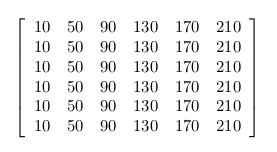
It looks like:

By convention 0 corresponds to black and 255 (8 bit representation) to white. For coloured image, we would have three 2D matrices or a single 3D matrix. We will be having one matrix for red, one for blue and one for green, their different combination can construct various colours. Only purpose of  camera is to collect photons coming from objects, depending on it, a number is assigned to each pixel.

Image Transformations

Transformation is a function that performs mapping from one set to another set after performing some operations. In image processing, there are six fundamental transformations:

1. Image Translation: Shifting the image in x or y direction. Let  be pixel in transformed image corresponding to  in input image. is required number of pixel translation. For y direction assuming similar notation:

   

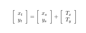
   Equation 1

   This kind of mapping suffers from one major drawback. It is very likely that some of the pixels in target/output image would remain unassigned as we are taking all pixels from the source/input image and then transforming them. This doesn’t ensure that all pixels in the target image would be assigned some value. This can be seen in following example:

   
   We can clearly see lots of holes in the output image. To solve this, inverse mapping is done. Each pixel from target image is taken and corresponding pixels in source image is computed using inverse mapping and in case, we get fractional pixel as result of the mapping, then, various interpolation techniques may be used.
   Translation along  x direction: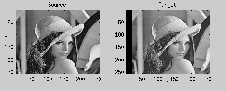

   

2. Image Rotation: Rotating the image in clockwise or counter clockwise by some angle around any pixel (usually done around image center). Using the concept of vector algebra, the rotation matrix can be easily derived:

   

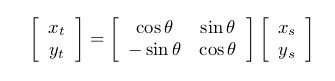
   Equation 2

   Following is an example of image rotation, in which the tilt in ‘Leaning tower of Pisa’ is corrected using image rotation. For better result, rotation can be done about center  pixel.

    

   

   Input Image

   

   Corrected Image
3. Image Scaling/ Zooming : Zooming feature in cameras is achieved using scaling. It is called digital zooming. It is different from optical zoom, where high power lenses are used to get high resolution image providing better clarity and scaling of the image. In digital zoom, the same information is mapped to canvas of higher spatial resolution. As a result of it, clarity of image is lost and we obtain a blurred image.
   Mathematical model of scaling: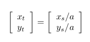

   

   Equation 3

   For a > 1, we have zoom out feature and for a < 1 zoom in.
   Example 1: Zoom In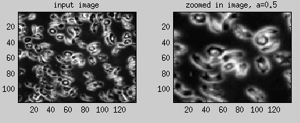

   
   Example 2: Zoom Out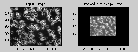

   

4. Shearing/Slanting: It is similar to shear effect observed in object when acted by a tangential force across one of its surface keeping the other surface fixed. In image processing, it is very useful in visualising shadow effects. Following figure shows shearing effect in x direction:
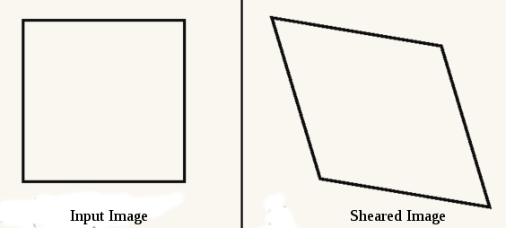
   Mathematical model for this is: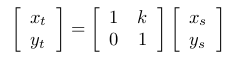

   

   Equation 4

   Here k decides the amount of shift in the position of the edge.

5. Affine Transformation: Affine transformation has 6 parameters and depending upon their values, we can have translations, rotations, scaling, slanting or combination of all.

   

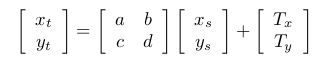
   Equation 5

   a,b,c,d, , are the deciding parameters.

6. Projective Transformation: As the name suggests, it deals with projections like mapping a 3D point to plane, or projecting a line in one plane to another plane oriented in different direction.
   1. Perspective Projection of 3D point on image plane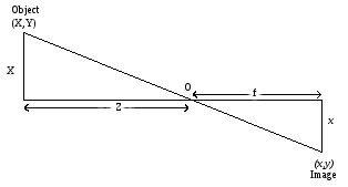
   Here, (X,Y,Z) is point in real world which is mapped to (x,y) in image plane and f
   is focal length of pinhole camera. From image,
   
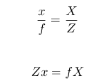
   Similarly,
   And,

   

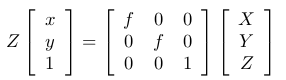
   Equation 6

   Here, Z is simply a scaling parameter as in an image only (x,y) matter and the depth information is lost. In short, , where, and are in image world and real world respectively.
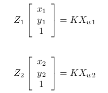
   This concept can be further extended for plane to plane transformation and homography.

   2. Plane to Plane Transformation
   Say P has image coordinate () when seen from (camera 1 position & has coordinate with respect to it) and image coordinate () when seen from (camera 2 position & has coordinate with respect to it). So, in totality we have two images of a scene taken from two points. Now we know:

   

   Equation 7 & 8

   Let and be related by some rotation (R) and translation (T):

   

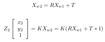
   Equation 9 &10

   From equation of plane, , where n is a vector normal to first image plane.

   

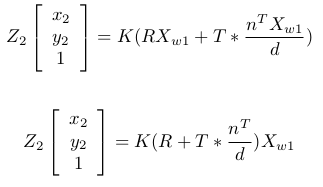
   Equation 11 & 12

   Using equation [7],

   

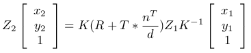
   Equation 13

   Doing some simplification, renaming :

   

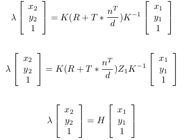
   Equation 14, 15 & 16

   H is the homography matrix and it relates images of same point in two different images.
   The H matrix has following structure: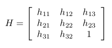

   

   Equation 17

   In order to estimate H, we need 8 equations. Hence, at least, 4 pairs of correspondence points are required from both images.

Image Registration

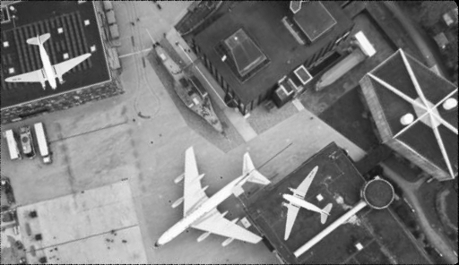
Image registration is process of using image transformation techniques in order to get an more workable image. Hence, it is usually the starting step in most image processing applications. Consider, the following two images of same view but taken at different time and from different view. Our job to find the difference between both images. Intelligent surveillance systems have this problem at their core i.e ability to find difference in consecutive frames from the images.

 

In its most simplified form, for camera motion constrained to a plane, we should be able to find at least two pixels corresponding to each other in both images to solve the problem. In general case, we have 6 degree of freedoms in camera motion and it would require knowledge of at least 4 pixels in both image as explained in previous section. In practical cases, problem may be a bit different, instead of point correspondences, we may have camera motion information. Camera motion information can directly give the rotation and translation parameters. Assuming pixel A(125,30) and B(373,58) in image 1 correspond to A'(249,94) and B'(400,329) in image 2. Using these, the governing equation is solved for , and and we obtain the registered image:

And difference between images can be found using algebraic difference between them.

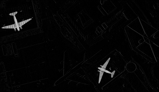
Image Mosaicing

Image Mosaicing commonly known as paranoma feature in phone cameras, is the alignment and stitching of a collection of images having overlapping regions into a single image.
Steps of Image Mosaicing (assuming we have 3 images, ):

1. Finding Homography between image pairs:
   As explained in Image Transformations section we need to find at least 4 pair of correspondences in a pair of images. In this case, assuming as reference we need to find such that and such that . The basic requirement for this is knowledge of the 4 pairs of point correspondences in between images. This is done using SIFT (space invariant feature transform). Using SIFT we get a large number of point correspondences say set containing points from image 1 and set containing points from image 2 corresponding to each point in set . We randomly select any 4 point correspondences from and  and solve the equation [16] to compute H matrix. Then, we check its performance using the computed H matrix by determining the correspondences for remaining points (point in =H* point in . We then select another set of 4 point correspondences and repeat the process. After repeating this for predetermined number of iterations, we choose that H matrix which gives the best performance.
   Read more about SIFT [2].
2. Creating the final combined image.
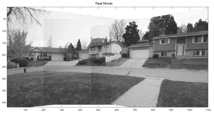
   After estimating the homography, we need to create an empty canvas. Center of canvas should be properly chosen to get the full mosaic. For every pixel in the canvas, we compute corresponding points in ,  and  using , identity matrix and respectively. That pixel can be assigned average of the obtained three values.

 

Input images:

 

The final mosaic is:

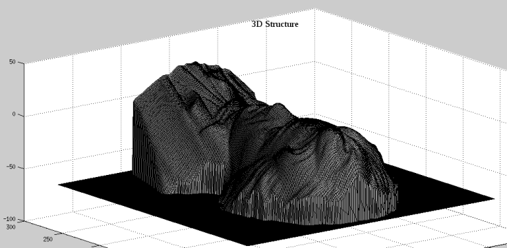
3D Reconstruction from Images

Another application of image processing techniques is in creation of 3D structure of objects using images.

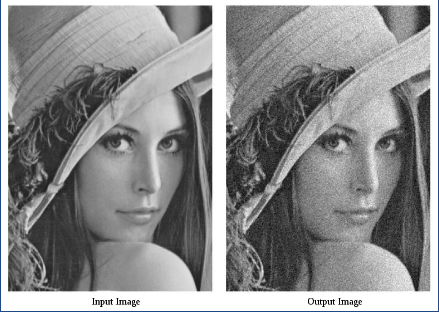
1. Depth Map from Blur
   Blur is usually considered as bad thing in images.There is nothing worse than a sharp image of a fuzzy concept. – Ansel AdamsBlur can occur in images either because of motion (camera or scene) or because of improper focus of scene.
   i) Motion Blur: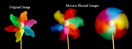ii) Defocus Blur:

 

Defocus blurred images have information related to depth of scene from the camera. In order to estimate the depth map of object, a series of images of the object are taken after moving it towards/away from camera in each image. Since, the object is 3D, not all points are in focus in a single image.

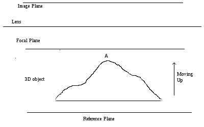
As shown in figure, if tip of object (A) is at its starting point, no point of object is in focus, but as object is moved towards camera, some portion of object start to come in focus and continue to be in focus in some images and as the whole object comes inside the range of focal length of camera, again, everything went out of focus. Using the taken images and information about the between images, the depth map can be easily computed.

How to find that some pixel is in focus or not?
This can be easily found by comparing the intensity at the pixel in all images, the one with maximum would be having that pixel in focus.

Once, we are able to relate each pixel with its focused image, relative depth can be easily mapped. Say in image point X is in focus and in image point Y is in focus, then the relative depth between X and Y is (10-4)* . This can be done for all points to find the complete depth map.

 

2.  Photometric Stereo:
This uses the images of same object taken under different lighting conditions to estimate its structure. Intensity observed for a particular pixel is function of angle between the light source and surface normal at corresponding point in the object. Hence, if we know the direction of illumination (position of light source) and intensity at the pixel, the surface normal can be obtained. This is done using singular value decomposition (SVD).
Check [3] for better understanding of SVD.

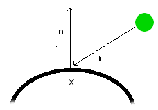
For intensity at any pixel (x,y):

 

Equation 18

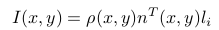
I is the intensity, is albedo (constant for the image), is the surface normal (unit vector) and is direction of light source.
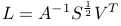
For k images each with size m x n, the above equation can be written as (taking as N):
Size of I would be mn x k, each image is having m*n pixel and there are total k images. N has size mn x 3, as each pixel has some normal and having 3 components (). Similarly, light source has 3 components () and there are k light sources as each image is corresponding to one light source. Hence, dimension of L is 3 x k.
Example:
Assuming we have 3 input images corresponding to 3 different illumination.

 

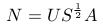
 We need to decompose I using SVD.

Equation 19

Size of S is mn x k, but size of N is mn x 3. A simple rank 3 approximation can resolve this.

Equation 20 & 21

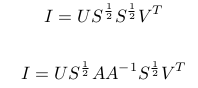
Here, A is ambiguity matrix.

Equation 22

Equation 23

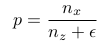
Next step is to compute surface gradient from N. Let p and q be defined as :

Equation 24

Equation 35

is just to avoid division by zero.
Using poisson solvers, we solve , ( g is the gradient g=[p q]) to obtain the 3D mesh of the object.

Conclusion

We have presented a mere glimpse to the vast, complex yet enchanting world of image processing. Basics of image processing and simple applications have been briefly discussed. These are the building blocks of computer vision.As explained earlier, image processing finds immense applications in various fields and having knowledge of some of its core concepts always come handy.

Check out links given in next section for better understanding about image processing and feel free to contact administrators for clarification/ discussion about the concepts mentioned in the article.

Learn more about Image Processing here:

[1] Coursera Online Courses:

1. Image & Video Processing: From Mars to Hollywood with a Stop at the Hospital
2. Fundamentals of Digital Image & Video Processing

[2] More about SIFT

[3] More about SVD

[4] The featured image is work of Kevin D. Jordan. Visit  the ultimate guide for editing milky way image  for learning more about image processing software ‘Lightroom’.